Designing a Real Portfolio Management System (Not a Positions UI)
Investment books, cash ledgers, reconciliation and the architecture behind reliable portfolio management.
Portfolio management looks like a UI problem. In practice it’s a truth problem: keeping positions and cash in a state that can be rebuilt day by day, backwards, deterministically.
A real failure mode: a custodian reports transactions with a different value date than trade date. In a “simple holdings table + dashboards” setup, NAV starts drifting, cash no longer matches the custodian, and performance is computed off the wrong base. A week later you don’t know whether the bug lives in the data, the logic, or the reconciliation.
This post lays out an architecture that removes that class of chaos: RAW → BOOK → VIEWS, a cash ledger as the source of truth, and reconciliation as a workflow (tolerances + reason codes), not a spreadsheet comparison.
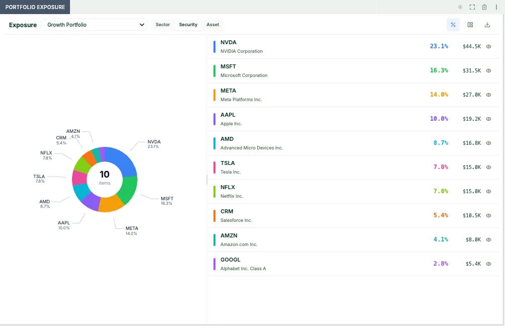
This post explains why each component exists, what failure mode it prevents, and includes concrete code snippets for the tricky parts.
The problem: most “portfolio management” products are just a UI on top of positions
Positions are the output. A real setup needs a pipeline that turns conflicting, messy inputs (custodians, corporate actions, FX, accruals) into a single auditable state.
If you’re designing this from scratch, dashboards are not the hard part. The hard part is designing truth.
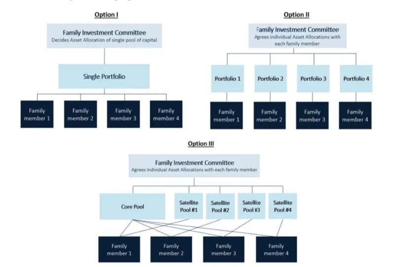
1. Three layers: Entity, Account, Portfolio
Portfolio is not an account. Most simple systems collapse everything into one “portfolio”, which works fine when you have one person and one broker account. That breaks immediately in real-world setups.
Entity = legal / tax owner
Examples: “Smith Family Trust 2020”, “Smith Holding GmbH”.
Holds tax identifiers, jurisdiction, household structure—needed for reporting and compliance.
Account = custody / brokerage account (where reconciliation happens)
Examples: “IBKR U1234567”, “JPM Custody #98765”.
Custodian feeds define positions/cash/transactions as they see them.
Portfolio = logical investment view / mandate
A portfolio can combine multiple accounts, represent a sleeve of one account, or be a model replicated across clients.
Example:
Entity: “Smith Family Trust”
Accounts: IBKR main + JPMorgan fixed income + Swissquote cash
Portfolios:
“Aggressive Growth” → 70% IBKR + 30% JPM
“Tech Sleeve” → only 40% of the IBKR account
“Conservative Income Model” → template used for several clients
Why it matters:
Tax follows entities
Cash & positions follow accounts
Investment decisions, attribution, constraints happen at portfolio level
2. Define “truth” before you write code
A portfolio system is not “a holdings table”. It’s a pipeline that resolves multiple sources into one book.
A clean hierarchy looks like this:
RAW custodian snapshots (immutable external truth)
BOOK (your reconciled book of record) (what you stand behind)
Portfolio views (sleeves/mandates/models derived from BOOK)
Derived analytics (NAV, P&L, returns, exposures)
If you start from (4) and work backwards, it will look correct—until reconciliation, FX, timing, and corporate actions show up.
3. Instrument vs Listing: stop storing “tickers” as identity
You don’t own “tickers”. You own instruments, and those instruments have listings. The same company (Apple) can trade on NASDAQ in USD, on XETRA in EUR, as an ADR in London, etc. If you store everything under one “symbol”, history breaks every time the ticker changes or a merger happens.
Instrument (global identity)
ISIN / FIGI, issuer, asset class, corporate action history lives here.
Listing is where/how it trades:
listing_key = (instrument_id, MIC/venue, currency, local_symbol)
This prevents ticker changes, dual listings, and currency variants from corrupting history.
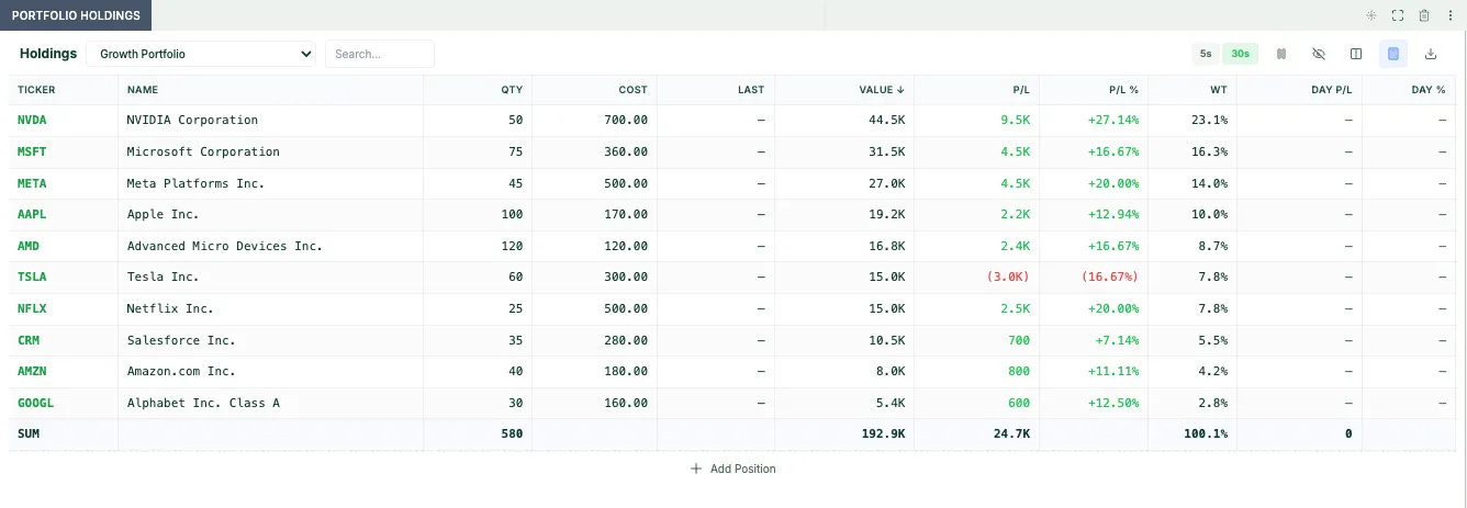
4. Cash ledger is the table that prevents silent NAV drift
Cash ledger invariants (non-negotiable):
Idempotency:
(source, external_id)is unique → re-imports never duplicate cash.Deterministic as-of:
BOOK(t)depends only on data ≤ t and explicit rules (FX, CA, accrual).Every transaction has a cash footprint: trades, fees, dividends, taxes, interest — all land in
cash_ledger.
Minimal schema:
cash_ledger(date, value_date, account_id, ccy, amount, type, external_ref, batch_id, status)
Cash forecast:
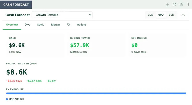
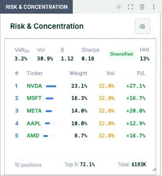
and risk & concentration:
5. Reconciliation is the product
Reconciliation is not a report — it’s a workflow. A reconciliation break should be a record with structure:
break_type(position | cash | fx | accrual)expectedvsobserved(with units + identifiers)tolerance_rule_id(absolute/relative thresholds)reason_code(missing_trade, wrong_fx, late_corp_action, etc.)status(open → investigated → resolved)maker/checker(auditability)
Without this, reconciliation collapses into ad-hoc spreadsheets and tribal knowledge.
6. Corporate actions: the graveyard of portfolio systems
Splits, spinoffs, mergers, tender offers, symbol changes—these require:
adjusting lots / basis allocation
creating new instruments
generating cash entries where applicable
mapping to custodian postings
supporting reprocessing
Pragmatic approach:
early phase: rely on what the broker already posted (transactions + cash)
store corporate actions as reference/justification
later: build a CA engine only when you have operational maturity
Trying to be “fully correct” on day one is how teams never ship.
7. Performance math: TWRR vs MWRR (IRR)
Returns: TWRR vs MWRR (and the convention that makes them well-defined). There are two standard ways to compute portfolio performance:
TWRR (Time-Weighted Rate of Return): measures the performance of the strategy/manager, neutralizing the timing and size of external cash flows.
MWRR (Money-Weighted Rate of Return / IRR): measures the investor’s realized return, including the impact of when cash was added/withdrawn.
The key is to make your cash-flow and NAV convention explicit.
Let:
NAV_t= end-of-day net asset value at timet(after pricing, accruals, etc.)F_t= external net flow for dayt(deposits - withdrawals).
(Trades are internal and are reflected in holdings/cash; they are not external flows.)
Assume NAV_t is measured after applying day t external flows (EOD booking). With this convention:
If an investor deposits cash on day
tand you book it on dayt, then that deposit appears inF_t, and it increasesNAV_tbut should not be counted as “return”.
TWRR (daily series, then compounding)
Daily TWRR return:
NAV timing matters (common production failure mode).
This equation assumes that NAV_t is measured after cash flows at time t. If your system measures NAV before flows, the formula must be adjusted accordingly.
Always define whether NAV is “pre-flow” or “post-flow” at each timestamp to avoid systematic but hard-to-detect performance errors.
Cumulative TWRR over days 1..T:
This is the standard “remove the external flow, then compute return”.
Edge cases / practical rules
If
NAV_{t-1} = 0(portfolio just started), TWRR is undefined for that day. Treat that period as “not invested yet” and start TWRR onceNAV_{t-1} > 0.If you have intraday flows, either:
aggregate to daily
F_twith a strict cutoff and keep this daily convention, orcompute sub-period returns around each flow time (more accurate, more complex).
Fees:
External fee paid out of portfolio (e.g., advisory fee withdrawn): treat as an external flow (reduces NAV but is not “market return”).
Internal trading costs/commissions: keep inside holdings/cash; they naturally reduce return.
MWRR (IRR on dated cash flows)
MWRR is the IRR of the investor’s cash flows.
Define a sequence of cash flows at exact times t_i (in years or day fractions):
Deposits into the portfolio: negative cash flow (investor pays in)
Withdrawals from the portfolio: positive cash flow (investor receives out)
For MWRR (XIRR), cash flows must include the terminal NAV as a final cash flow at time TTT. The NAV is treated as a positive cash flow occurring at the valuation timestamp.
So you solve for r in:
where Δti is the time (in years) from tit_iti to the end time T (or use a consistent base date; just be consistent).
Interpretation:
MWRR answers: “Given when I put money in and pulled money out, what annualized return did I personally experience?”
It will differ from TWRR when flows are timed into/out of good/bad market periods.
Practical implementation details
Use actual day counts for Δti (e.g., ACT/365 or ACT/360). Pick one and document it.
If you compute period MWRR (e.g., month), include all flows in that month plus terminal value at month-end.
If multiple flows happen on the same day, sum them (or keep separate; both work).
Relationship: what each metric is for
Use TWRR to compare managers/strategies and to attribute performance to positions/factors.
Use MWRR to report what the investor actually earned and to explain “why my experience differs from the strategy’s performance”.
def twrr_from_daily_nav(daily_nav: pd.Series, flows: pd.Series) -> float:
    """
    daily_nav: Series indexed by date (EOD NAV in base currency)
    flows: Series indexed by date (external flows; +deposit, -withdrawal)
           Convention: NAV_t includes flow_t (flow booked at EOD).
    Returns: total TWRR as a decimal (e.g., 0.1846 = +18.46%)
    """
    daily_nav = daily_nav.sort_index()
    flows = flows.reindex(daily_nav.index, fill_value=0.0)

    nav_prev = daily_nav.shift(1)
    # Return factor for day t: (NAV_t - flow_t) / NAV_{t-1}
    factor = (daily_nav - flows) / nav_prev
    factor = factor.dropna()

    return float(factor.prod() - 1.0)

# Example (explicit, internally consistent):
# Jan 1: 100k
# Jan 15: NAV 130k after adding 20k at EOD (so NAV includes the flow)
# Jan 31: 140k
nav = pd.Series(
    [100_000, 130_000, 140_000],
    index=pd.to_datetime(["2026-01-01", "2026-01-15", "2026-01-31"])
)
flows = pd.Series(
    [0, 20_000, 0],
    index=pd.to_datetime(["2026-01-01", "2026-01-15", "2026-01-31"])
)

print(f"TWRR: {twrr_from_daily_nav(nav, flows)*100:.2f}%")
In production you do this after:
converting multi-currency positions/cash to a base currency using consistent daily FX
deciding how you treat settlement/value dates (critical for fixed income and cash)
MWRR / XIRR (robust version)
Cash flow list:
For each external flow on date/time
d:CF = -flow_amount(deposit negative, withdrawal positive by investor sign convention; choose one and keep consistent)Add terminal flow at end date/time
T:CF_terminal = +NAV_T
Then solve IRR via Newton-Raphson (with bisection fallback for robustness).
Robustness rules:
If all cash flows have the same sign → IRR is undefined.
If Newton fails (derivative near zero / diverges), fallback to bisection on a bracket like
[-0.9999, 10](or wider if needed).
from scipy.optimize import newton

def xirr(cashflows):
    """
    cashflows: list of (date, amount)
    amount: negative for contributions, positive for withdrawals and terminal value
    """
    dates = pd.to_datetime([d for d, _ in cashflows])
    amounts = np.array([a for _, a in cashflows], dtype=float)

    t0 = dates.min()
    years = (dates - t0).days / 365.25

    def f(r):
        return np.sum(amounts / (1 + r) ** years)

    def fprime(r):
        return np.sum(-years * amounts / (1 + r) ** (years + 1))

    return float(newton(f, x0=0.05, fprime=fprime, maxiter=100))

# Example:
# Invest 100k on Jan 1, add 20k on Jan 15, end value 140k on Jan 31
cashflows = [
    ("2026-01-01", -100_000),
    ("2026-01-15", -20_000),
    ("2026-01-31", 140_000),
]

print(f"MWRR (XIRR): {xirr(cashflows)*100:.2f}%")